Pause live data, measure a change, and compare two runs

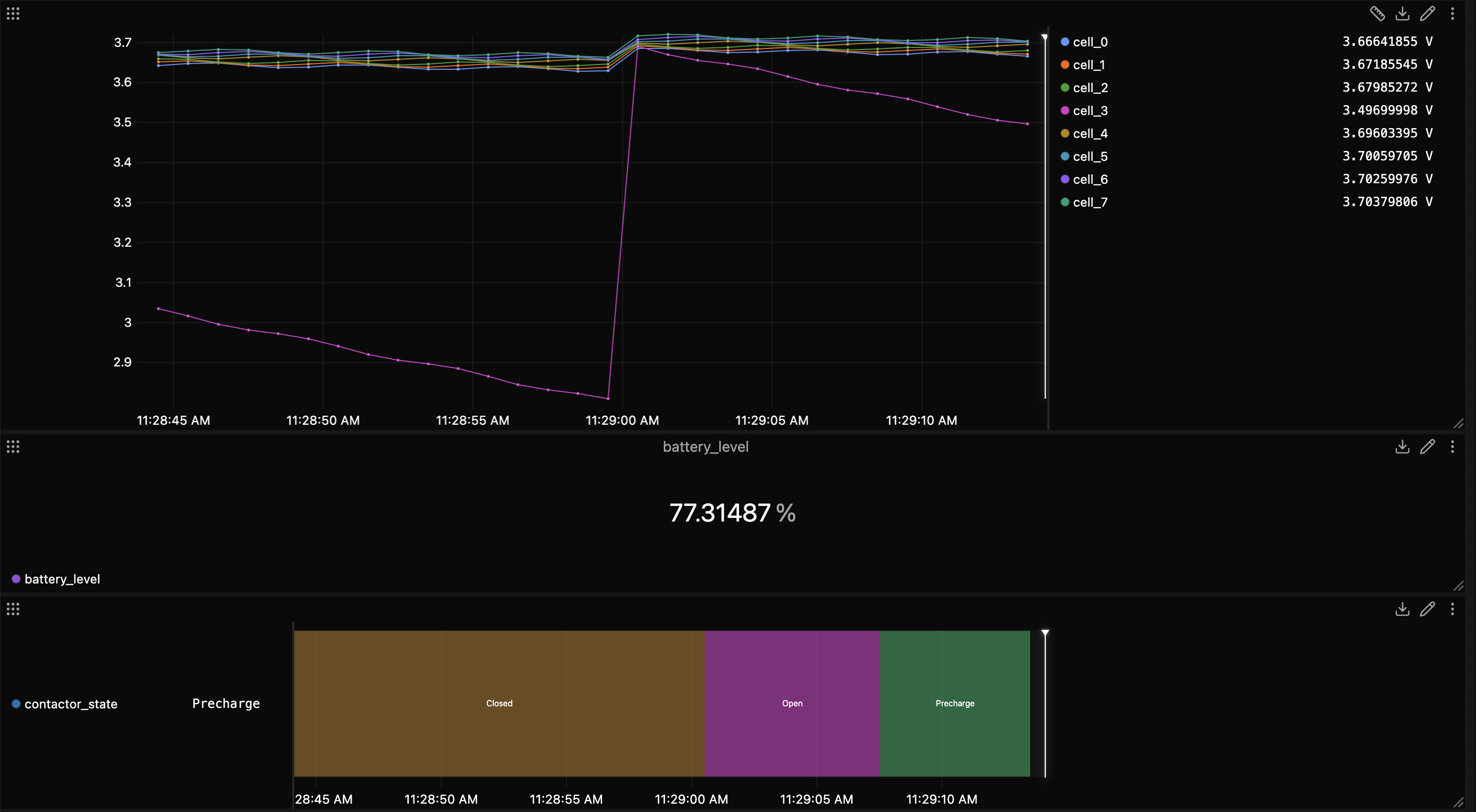
A cell voltage dips on a live plot, and by the time you look, it has scrolled away. This guide stops the view on that moment, measures the drop, saves the run, and lays it over a second run. In this example, one cell (cell_3) dips under 3.0 V near the end of every minute.

This guide runs on simulated data. Install the CLI shows how to start it.

Pause holds the view while the agent records

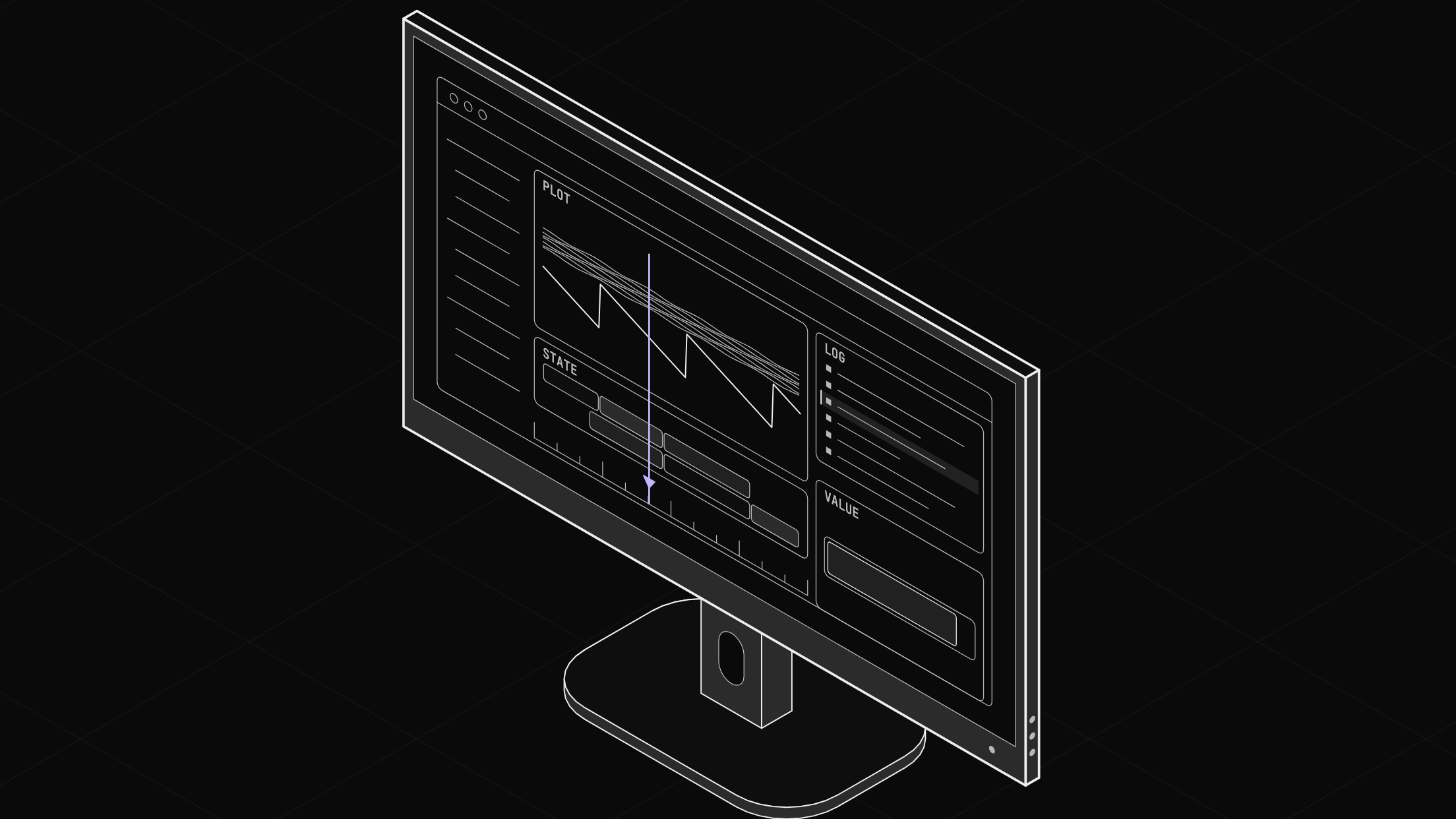
While live, a tab follows the newest data over a sliding window, 30 s by default. When you pause, the tab holds still on one cursor, and every panel reads its value there. The agent keeps recording.

The app drawn on a monitor: a plot of eight close cell lines, one sagging in a repeating sawtooth, over a state panel, with log and value panels beside it and one violet cursor line running down through the plot and state.

Before you start

The Zelos app.
A live tab with a plot.

Step 1: Pause

Choose Pause in the middle of the timeline bar, or press Space. The cursor lands on the newest sample, and the legend and the other panels read there. Choose Live or press Esc to follow live data again.

Live, then Pause: the legend and the panels read at the cursor.

The paused tab: the cell plot with a value beside each legend chip, and the other panels reading at the cursor.

Step 2: Move the cursor and zoom

Drag along the timeline, or right-click a plot, to move the cursor. Drag across a plot to zoom, double-click to go back, and choose Fit all (or press 0) to see all the data.

Scrub the timeline, right-click the plot, drag to zoom, double-click back, then Fit all.

Step 3: Frame the change and measure it

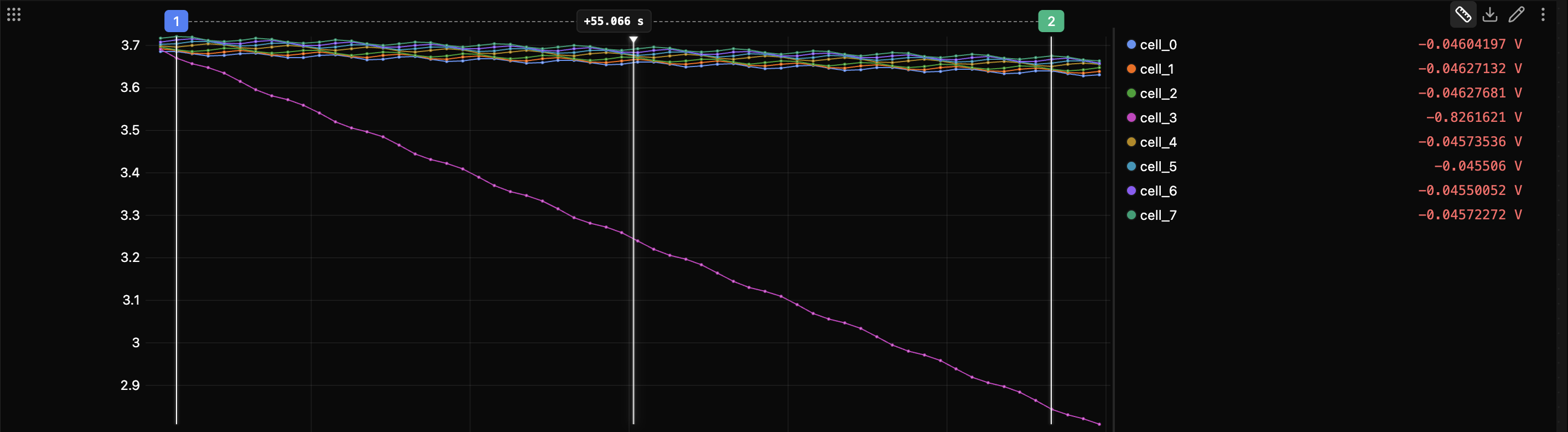
Right-click the plot where the change happens to move the cursor there. Then choose a window size in the view window menu at the left of the timeline bar, such as 1m. A paused view re-centers on the cursor, so the change sits in the middle of the window.

Choose the ruler, Measurement Tool, in the plot's header, and drag its two cursors out to the ends of the change. The bracket reads Δt, and each chip reads its signal's signed change. In this example, cell_3 fell 0.83 V and each of the other seven cells about 0.05 V.

The ruler across one minute: cursors 1 and 2, a time bracket, and a signed change beside each chip, -0.826 V for cell_3. — The ruler belongs to this plot only.

Step 4: Save the run

Choose Save trace, the disk icon at the right of the timeline bar, and type a name. Upload sends the run to Zelos Cloud, where your team can open it, on any plan. Export writes the run to a .trz file on this computer and needs a paid plan. This example exports to files: type cycle-1, choose Export, and pick a folder. A toast reads "Trace saved".

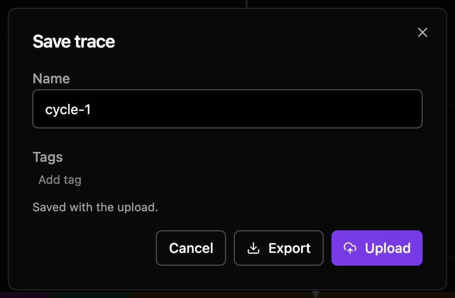
The Save trace dialog: the name cycle-1, a Tags row, and the Cancel, Export and Upload buttons.

Both save every signal in the window on screen. The file name becomes the run's label.

Save a second run the same way as cycle-2. Here it is the same window two minutes later.

Step 5: Open both runs

Tip: build the plot you want before you open the second trace. A signal added while two traces are open belongs to only one of them, so it draws only one run.

In Data on the right, choose Open trace, File, and pick cycle-1.trz. The tab leaves live and shows the file. Then choose Add trace, File, and pick cycle-2.trz.

Now each chip names its run first, cycle-1::cell_3 and cycle-2::cell_3, and the other panels show one reading per run. Relative time is on, so each trace starts at 0:00. Choose REL to switch to ABS and see the runs where they happened, then ABS to switch back.

Open trace, then Add trace. REL starts both runs at zero; ABS shows them where they happened.

Step 6: Read both runs at one moment

Right-click the plot where the change happens. In this example, near 47 s, both cell_3 chips read about 2.99 V, and their lines lie on top of each other.

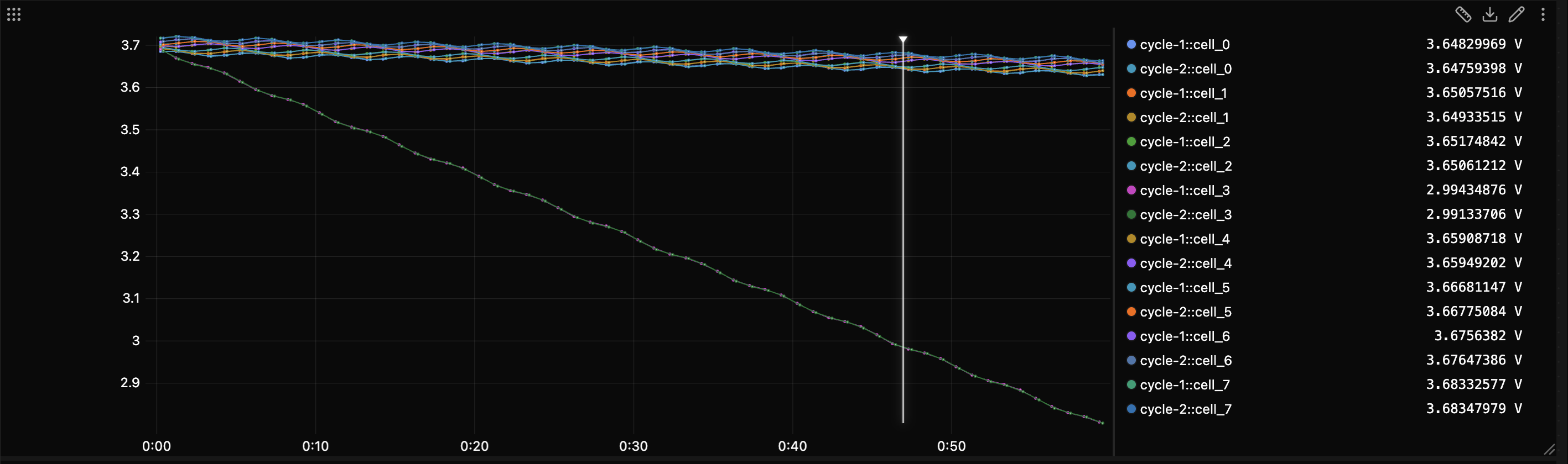
Both runs in relative time with the cursor near 47 s: the weak cell's two lines coincide, and its two chips read 2.994 V and 2.991 V. — Both runs at 0:46.951, on an axis of elapsed time.

The simulated cell voltages repeat every 60 seconds, so these two lines match. On your bench, the gap between the lines is the change you look for.

Where this trips people up

A tab shows either live data or traces. To go back to live, choose the agent's row under Recent in Data.
The ruler works only while paused.

Next: save the layout

Build a view once and reuse it on every run keeps these panels for the next run. Turn a notebook into a pass/fail test fails a run on the same dip. The timeline reference lists every control, and multi-trace mode covers more runs.